International Baccalaureate Mathematics

Syllabus Content

The normal distribution and curve. Properties of the normal distribution. Diagrammatic representation. Normal probability calculations. Inverse normal calculations

Here are some specific activities, investigations or visual aids we have picked out. Click anywhere in the grey area to access the resource.

Normal Distribution Calculator A customised online calculator for quickly finding areas under the normal distribution curve.

Here are some exam-style questions on this statement:

"The heights of palm trees along a beach are normally distributed with a mean of 4.55m and a standard deviation of 0.37m." ... more

"A group of students sat a Biology examination and a Computer Studies examination. The students' marks in the Biology examination are normally distributed with a mean of 70 and a standard deviation of 9." ... more

"The time in minutes taken to drive through a city at different times of the day can be modelled by a normal distribution with mean of 45 and standard deviation of 12. A commuter will be late for work if it takes more than an hour to drive through the city." ... more

"The heights, H metres, of flowers called Xylothorn Blooms growing in the dense forests of Verdantem on the luminous planet Aurorion can be modelled by a normal distribution with mean 14.3 metres and standard deviation 3.9 metres." ... more

"A random variable $X$ is normally distributed with $\mu=250$ and $\sigma=25$." ... more

"The weights in grams of 98 mice are shown in the cumulative frequency diagram. The heaviest mouse weighted 160g." ... more

"The weights of players in a sports league are normally distributed with a mean of 75.2 kg, (correct to three significant figures). It is known that 75% of the players have weights between 67 kg and 80 kg. The probability that a player weighs less than 67 kg is 0.05." ... more

"Eels are elongated fish, ranging in length from 5cm to 4m. In a certain lake the length of the eels are normally distributed with a mean of 84cm and a standard deviation of 18cm. Eels are classified as giant eels if they are more than 120 cm long." ... more

"The length, $X$ minutes , of a certain category of online video is normally distributed with a mean of 28." ... more

"The length of Costlow's bâtard bread loaves in centimetres is normally distributed with mean $ \mu $. The following table shows probabilities for values of $L$." ... more

See all these questions

Click on a topic below for suggested lesson Starters, resources and activities from Transum.

Probability Probability is a measure of the weight of evidence, and is arrived at through reasoning and inference. In simple terms it is a measure or estimation of likelihood of the occurrence of an event. The word probability comes from the Latin word probabilitas which is a measure of the authority of a witness in a legal case. Some of the earlier mathematical studies of probability were motivated by the desire to be more profitable when gambling. Today however the practical uses of probability theory go far beyond gambling and are used in many aspects of modern life. We believe that even adults can, in many cases, have a poor intuition regarding the effects of probability. These activities are designed to help pupils calculate but also get a 'feel' for the principles of probability.

Furthermore

Official Guidance, clarification and syllabus links:

Awareness of the natural occurrence of the normal distribution.

Students should be aware that approximately

$ \quad 68$% of the data lies between $ \mu \pm \sigma$

$ \quad 95$% lies between $ \mu \pm 2\sigma$

$ \quad 99.7$% lies between $ \mu \pm 3\sigma$.

Probabilities and values of the variable must be found using technology.

For inverse normal calculations mean and standard deviation will be given.

This does not involve transformation to the standardized normal variable z.

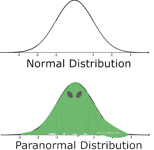
The normal distribution is a continuous probability distribution that is symmetrical around its mean, representing a bell-shaped curve where the bulk of the values lie close to the mean. The standard normal distribution has a mean of zero and a standard deviation of one. It is crucial in statistics because of its natural occurrence in various natural phenomena and its use in inferential statistics.

The key formula for the normal distribution is its probability density function (PDF):

$$ f(x | \mu, \sigma^2) = \frac{1}{\sqrt{2\pi\sigma^2}} e^{- \frac{(x - \mu)^2}{2\sigma^2}} $$

Where:

$ \mu $ is the mean of the distribution,
$ \sigma $ is the standard deviation,
$ \sigma^2 $ is the variance,
$ x $ is the variable,
$ e $ is the base of the natural logarithm.

An example of the normal distribution in use is finding the probability that a randomly selected value is less than a certain number. For instance, if the mean score of an exam is 60 with a standard deviation of 10, what is the probability of a student scoring less than 75?

$$ P(X < 75) = \int_{-\infty}^{75} \frac{1}{\sqrt{2\pi \cdot 10^2}} e^{- \frac{(x - 60)^2}{2 \cdot 10^2}} \, dx $$

This formula would never be required in an exam. Students need to be proficient in using the GDC for calculations involving the normal distribution that go beyond simple situations.

If you would like to interact with the graph of the standardised normal distribution you will find it waiting for you on the Graph Plotter.

The equation is:

$$y = \frac{1}{\sqrt{2\pi}} e^{-\frac{x^2}{2}}$$

Students should be aware that approximately 68% of the data lies between within one standard deviation away from the mean, 95% lies between 2 standard deviations away from the mean and 99.7% of the data lies between 3 standard deviations away from the mean. This is one of of those facts that needs memorising.

If you would like to interact with the graph of the normal distribution you will find it waiting for you on the Graph Plotter page (you will need to rescale the axes).

If you use the TI-Nspire calculator you can find instructions for using the Normal CDF function on the GDC Essentials page.

This Normal Distribution video is from Revision Village.

This Bicen Maths video clip shows everything you need to memorise on this topic for A Level Statistics.

How do you teach this topic? Do you have any tips or suggestions for other teachers? It is always useful to receive feedback and helps make these free resources even more useful for Maths teachers anywhere in the world. Click here to enter your comments.

International Baccalaureate Mathematics

Statistics and Probability

Furthermore